Sampling and Weighting Technical Report, Census of Population, 2021
7. Statistical inference
Statistical inference in the context of survey sampling is the process of drawing conclusions about the population based on data collected from survey respondents. To draw conclusions about the target population of the long-form sample survey using estimates produced from the sample, the uncertainty of these estimates must be taken into consideration. As described in Chapter 6, estimates produced from the long-form sample are subject to variability because of sampling and non‑response. The variance of each estimate is a measure that quantifies this variability. Estimates of the variance of survey statistics can be used to produce other measures of the quality of the statistics that reflect their variability, but are more easily interpreted than the variance estimates themselves. These measures include standard errors, coefficients of variation and confidence intervals. Among these measures, confidence intervals have the advantage that they allow users to easily perform statistical inferences. For this reason, the confidence interval was chosen as the variance-based quality indicator to accompany long-form estimates for the 2021 Census.
7.1 Confidence intervals and their interpretation
A confidence interval for an estimate is an interval constructed around the estimate that reflects the estimate’s uncertainty. A confidence interval is associated with a confidence level, which is expressed as a percentage. The confidence level describes the degree to which one can be confident that the true population parameter is contained in the confidence interval. A default confidence level is generally set for a survey or in a field of study based on user needs. A commonly used confidence level is 95%, and this is the default confidence level for the census dissemination system. Given an estimate together with a 95% confidence interval for the estimate, a user can infer with 95% confidence that the true population parameter is contained within the interval.
A rigorous interpretation of confidence intervals relies on hypothetically repeating the sampling and estimation procedures. This interpretation is illustrated in Figure 7.1.1.
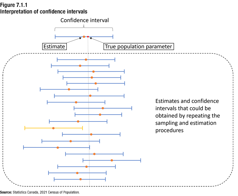
Description for Figure 7.1.1
At the top of Figure 7.1.1 is a horizontal line representing a confidence interval. An orange dot is marked near the centre of the line to represent the estimate of the population parameter. To the right of the orange dot, a red dot is marked on the line to represent the true population parameter.
There is a large box below the confidence interval containing 20 similar horizontal lines representing different confidence intervals. The horizontal position of each of these 20 confidence intervals is different, and the lengths of the confidence intervals vary somewhat as well. Near the centre of each of the 20 confidence intervals is an orange dot, indicating the estimate of the population parameter. These 20 estimates and their corresponding confidence intervals represent the estimates and confidence intervals that could be obtained by hypothetically repeating the sampling and estimation procedures 20 times.
A vertical line extends downward through the diagram from the true population parameter depicted in the confidence interval at the top of the diagram. This line serves to indicate whether the true population parameter is contained in each of the 20 different confidence intervals. The confidence intervals intersecting the vertical line contain the true population parameter. Of the 20 confidence intervals, 19 are colour-coded in blue to show that they contain the true population parameter, while the remaining confidence interval is colour-coded in yellow to show that it does not contain the true population parameter.
Source: Statistics Canada, 2021 Census of Population.
Full description:
The top part of Figure 7.1.1 depicts a confidence interval for the estimate of a population parameter. This particular confidence interval contains the true population parameter.
The figure also shows different estimates that could be produced by hypothetically repeating the sampling and estimation procedures several times, together with their corresponding confidence intervals. In the case of the long-form questionnaire, this repeated sampling and estimation would involve drawing a very large number of samples from the long-form sample universe according to the sampling design described in Chapter 2. Each one of the samples would undergo the same processing, weighting and estimation steps as the actual sample. The estimates and the confidence intervals produced for a given characteristic would generally be different for the different samples. However, if the underlying assumptions of the given confidence interval method are valid, the percentage of the confidence intervals that contain the true population value would be approximately equal to the confidence level.
In the example depicted in the figure, all but one of the confidence intervals contain the true population parameter.
The width of the confidence interval for an estimate is an indication of the degree of uncertainty of the estimate. If two estimates are equal, but one has a wider 95% confidence interval than the other, then the estimate with the wider interval has greater uncertainty.
The types of uncertainty reflected in the confidence intervals for long-form estimates differ according to the stratum type. Since confidence intervals are based on variance estimates, they reflect the same types of uncertainty as the underlying variance estimates. In mail-out, list-leave, and mail-out with drop-off collection units (CUs), where the sampling fraction is one-quarter, the uncertainty measured is due to sampling and total non‑response. In CUs in First Nations communities, Métis settlements, Inuit regions and other remote areas, where all households are sampled, the uncertainty measured is due only to total non‑response.
7.2 Constructing confidence intervals
Confidence intervals are generally based on the properties of a mathematical expression called a pivot. Depending on the pivot used and on which assumptions are made about the properties of the pivot, different types of confidence intervals will result from it. When constructing a confidence interval for a population parameter
,
the pivot used will typically involve the estimate of theta, denoted by
,
and the standard error of
.
The standard error of an estimate is defined to be the square root of the estimated variance of the estimate. The standard error of
is denoted by
.
The pivot may also involve additional quantities. The most commonly used type of confidence interval, the Wald interval, is based on the following pivot:
The assumption underlying the Wald interval is that this pivot approximately follows a standard normal distribution, i.e., a normal distribution with a mean of zero and a standard deviation of one. The lower bound (LB) and upper bound (UB) of the 95% Wald confidence interval for the population parameter
are given by:
where
is the 97.5th percentile of the standard normal distribution.
In many situations, the assumption that the Wald pivot is approximately normal is not satisfied. When the assumptions underlying the construction of a confidence interval are violated, this can lead to undercoverage of the confidence interval. In other words, if the sampling and estimation procedures were repeated a very large number of times and corresponding confidence intervals were constructed for each estimate using the same method, the proportion of these confidence intervals containing the true population value could be less than the stated confidence level.
To minimize the risk of undercoverage, more advanced methods than the Wald construction have been used to produce the confidence intervals for long-form estimates. These methods are known to achieve coverage closer to the nominal rate. However, all methods of constructing confidence intervals rely on assumptions that are generally not possible to explicitly verify in specific use cases. When working with confidence intervals, data users should be mindful of the scenarios that can lead to violation of the assumptions underlying the confidence interval construction. The different methods used to produce confidence intervals for long-form estimates, as well as the required assumptions, are described in detail in the following sections.
7.3 Student’s confidence interval
The Student’s confidence interval is used for all long-form statistics except proportions and counts. Since most estimates disseminated for the long-form are in fact for proportion and count statistics, this method accounts for a minority of disseminated confidence intervals.
The Student’s confidence interval is based on the same pivot as the Wald interval. However, rather than assuming that the distribution of this pivot can be approximated by a normal distribution, the approximating distribution is assumed to be a Student’s t-distribution. This distribution is known to be a more suitable approximating distribution for the pivot in cases where the sample size is small. The Student’s t-distribution is specified by a single parameter known as the “degrees of freedom.” The number of degrees of freedom of the Student’s t‑distribution is influenced by the sampling design, the number of sampled units and the variance estimation method. The number of degrees of freedom affects the width of the confidence interval. For the 2021 Census, the degrees of freedom were approximated by the number of replicates used for variance estimation (see Section 6.2) and denoted by
.
The lower bound and the upper bound of a 95% Student’s confidence interval for a population parameter of interest
are given by:
where
-
is the estimate of
.
-
is the 97.5th percentile of the Student’s t-distribution with
degrees of freedom.
-
is the standard error of
.
7.3.1 Properties of the Student’s confidence interval
The Student’s t-distribution is nearly identical to a standard normal distribution when the number of degrees of freedom is very large. When the number of degrees of freedom is small, the Student’s t-distribution is wider than the standard normal distribution. This leads to the Student’s confidence interval being wider than the Wald interval for the same estimate. Wald intervals often suffer from undercoverage when the sample size is small. Although the census long-form has a large sample size for the entire country, the sample size in small geographic areas or small domains of interest may be small. The Student’s confidence interval will generally have better coverage than the Wald interval in these cases.
In practice, Student’s confidence intervals may still suffer from undercoverage for very small sample sizes. This is due to failure of the assumptions when the sample size is very small. For instance, the distribution of the pivot may not be well approximated by a Student’s t-distribution, or the approximation of the degrees of freedom by the number of replicates may substantially overestimate the actual degrees of freedom of the distribution. The breakdown of these assumptions when the sample size is very small will generally lead to undercoverage of the Student’s confidence intervals.
7.4 Modified Wilson confidence interval for proportions
There are several different methods for constructing confidence intervals for proportions. For the 2021 Census, the modified Wilson confidence interval method was chosen because of its generally superior coverage and its practicality for implementation. This method is used for all proportion-type statistics. The method is based on the Wilson confidence interval for a simple random sampling with replacement (SRSWR) sample design (Wilson 1927). For the census, a modified version of this confidence interval is used that has been adapted to complex sample designs (Kott and Carr 1997). Extensive simulation studies have shown that this method performs better than the Wald and Student confidence intervals in situations where those confidence intervals exhibit undercoverage for proportion-type statistics (Neusy and Mantel 2016; Statistics Canada 2023).
For proportions, the assumption that the pivot used to construct the Student’s confidence interval follows a Student’s t‑distribution breaks down for small sample sizes and when the statistic takes values near zero or one. The modified Wilson confidence interval for a proportion
is based instead on the following pivot:
where
-
is the estimate of
-
is the effective sample size
-
is the estimated design effect of
with respect to an SRSWR sample design
-
is the in-scope sample size
-
is the estimated variance of
.
The in-scope sample size is defined to be the number of sampled units which are in-scope for the question corresponding to the proportion
,
i.e., the number of sampled units for which the question is applicable and which belong to the population of interest for the question. The expression under the square root sign in the denominator of the pivot is the variance of the proportion estimate under an SRSWR sample design, but with the sample size replaced by the effective sample size. By using the effective sample size in this expression, the variance is adjusted to account for the complex sample design of the census long-form. The modified Wilson confidence interval is based on the assumption that this pivot approximately follows a Student’s t-distribution. As with the Student’s confidence interval, for the 2021 Census, the degrees of freedom of the Student’s t-distribution are approximated by
,
the number of replicates used for variance estimation.
The lower bound and the upper bound of a 95% modified Wilson confidence interval for the proportion
are given by:
where
is the 97.5th percentile of the Student’s t-distribution with
degrees of freedom and the other terms are as defined above.
7.4.1 Properties of the modified Wilson confidence interval for proportions
In addition to achieving better coverage than the Wald and Student intervals for small sample sizes and when the population parameter is near zero or one, the modified Wilson confidence interval for a proportion has the desirable property that its lower bound is never less than zero and that its upper bound is never greater than one. Since proportions cannot take on values outside of the interval between zero and one, it is reasonable that confidence intervals for proportions would exclude negative values and values greater than one.
It should also be noted that, unlike the Wald and Student intervals, the modified Wilson confidence interval for proportions is asymmetric, meaning that the estimate will not be exactly at the centre of the interval. The asymmetry is small when the effective sample size is large or when the estimated proportion is near 0.5.
Much like the Wald and Student confidence intervals, the modified Wilson confidence interval for proportions may suffer from some undercoverage, particularly when the sample size is very small, the value of the proportion is near zero or one, or there is high correlation between members of the same household. However, the modified Wilson method generally achieves nominal coverage rates in extreme situations, compared with the Wald and Student methods. It generally maintains coverage as good as or better than the Wald and Student methods in those situations.
7.5 Modified Wilson confidence interval for counts
For long-form estimates of counts, the confidence interval method used is a modified Wilson method similar to the method used for proportion-type statistics. For counts, the Wald and Student confidence intervals often perform poorly when the sample size is small, and when the value for the variable of interest is zero for almost all sampled units or when the value is one for almost all sampled units. In these situations, the distribution of the pivot used to construct the Wald and Student’s confidence intervals is generally not well approximated by either a normal distribution or a Student’s t-distribution.
The modified Wilson confidence interval for counts was developed for the 2021 Census as an alternative to the Wald and Student’s confidence intervals which achieves coverage closer to the nominal rate. It has been tested in a simulation environment similar to the census long-form and has been shown to typically achieve good coverage (Neusy et al. 2021).
7.5.1 Modified Wilson confidence interval for counts: Theoretical form
The version of the modified Wilson confidence interval for counts used for the 2021 Census is an approximation of a theoretical form of the interval. The theoretical form can be derived in a similar manner to the modified Wilson confidence interval for proportions. In the case of the modified Wilson confidence interval for counts, the formulation relies on the notion of a calibration group of interest. A calibration group is a collection of units for which survey weights are calibrated with respect to control totals (for the census long-form, the calibration groups are ADAs and SADAs), and a calibration group of interest for a count
is a calibration group that could potentially contain units with the characteristic of interest corresponding to
.
The modified Wilson confidence interval for a count
is based on the following pivot:
where
-
is the estimate of
-
is the total population size of the calibration groups of interest
-
is the effective total sample size in the calibration groups of interest
-
is the total sample size in the calibration groups of interest
-
is the estimated design effect of
with respect to an SRSWR sample design, with population and sample size terms based on the calibration groups of interest
-
is the estimated variance of
.
The population size and sample size terms are defined with respect to the calibration groups of interest because this leads to a confidence interval with good properties. Specifically, simulations show that the resulting confidence interval has better coverage than for alternative ways of defining the size terms (Neusy et al. 2021).
Similar to the modified Wilson confidence interval for proportions, the modified Wilson confidence interval for counts is based on the assumption that the pivot approximately follows a Student’s t-distribution. Like all confidence intervals for the 2021 Census, the degrees of freedom of the Student’s t-distribution are approximated by
,
the number of replicates used for variance estimation.
From the above pivot, the theoretical version of the 95% modified Wilson confidence interval for the count
can be derived. This version of the interval has the following lower bound and upper bound:
where the terms are as defined above. In this version of the interval, the similarity to the modified Wilson confidence interval for proportions is evident.
7.5.2 Modified Wilson confidence interval for counts: Approximate form
The approximate form of the modified Wilson confidence interval for counts that was implemented for the 2021 Census is based on the theoretical interval above. An approximation was used because of limitations of the census tabulation system.
In the approximate form, the lower bound and the upper bound of a 95% modified Wilson confidence interval for a count
are given by:
where
-
is the estimate of
-
is the 97.5th percentile of the Student’s t-distribution with
degrees of freedom
-
is the estimated variance of
.
7.5.3 Assumptions for approximating the modified Wilson confidence interval for counts
It has been demonstrated empirically that the approximation implemented for the census behaves well for sample designs similar to that of the long-form (Neusy et al. 2021). The approximation is based on the following assumptions:
- The total sample size in the calibration groups of interest
is sufficiently large so that
is close to zero.
- The estimated count
is much smaller than the total population size of the calibration groups of interest
.
The first assumption is generally valid for the census long-form questionnaire because the calibration groups of interest correspond to SADAs or ADAs, which always have a very large sample size. The second assumption may not be met, but only for common characteristics and for very large domains of interest, such as SADAs. In this context, the approximate version of the modified Wilson confidence interval is nearly identical to the Student confidence interval, and both methods perform well enough for large domain sizes. Therefore, not meeting the second assumption is not a concern for the census long-form.
7.5.4 Properties of the modified Wilson confidence interval for counts
The modified Wilson confidence interval for counts has the advantage over the Wald and Student confidence intervals that the lower bound of the confidence interval is never less than zero. This property, as well as the other properties described in this section, applies to both the theoretical and the approximate version of the confidence interval. Since count statistics cannot be negative, it is appropriate that the confidence interval does not contain negative values. Similarly to the modified Wilson confidence interval for proportions, the modified Wilson confidence interval for counts is asymmetric. This asymmetry will be small when the estimated variance of a count is small in relation to the estimated count itself.
Much like the Wald and Student confidence intervals, the modified Wilson confidence interval for counts may suffer from some undercoverage, particularly when the sample size is very small, the value of the count is close to zero or close to the size of the population of the domain of interest, or there is high correlation between members of the same household. However, the modified Wilson method generally achieves nominal coverage rates in extreme situations, compared with the Wald and Student methods. It generally maintains coverage as good as or better than the Wald and Student methods in those situations.
