Sampling and Weighting Technical Report, Census of Population, 2021
6. Variance estimation

The error in an estimate is the difference between the estimate and the actual value of what is being estimated. All estimates from the census questionnaires are subject to non‑sampling errors such as total non‑response error. Estimates from the long‑form questionnaire are also subject to sampling error. Sampling error stems from the fact that the estimates are based on observations from a sample and not from the Census of Population. Total non‑response error occurs when households selected in the sample do not respond to the survey.

The error in an estimate has a random component, measured by variance, and a systematic component, measured by bias. Variance measures how much the estimate varies from the average that would result from hypothetical repetitions of the survey process. Variance can be estimated using data from the sample. Bias is the difference between the average estimate that would result from hypothetical repetitions of the survey process and the actual value of the characteristic being estimated. The sampling and estimation methods used in the long-form sample survey all aim to minimize the bias.

Some estimation methods are more precise than others in estimating a particular characteristic of the population, so they can affect error. The estimated variance can be used to produce several quality indicators that are often used to measure the accuracy of an estimate. For example, it can be used to calculate standard errors, confidence intervals and coefficients of variation. The confidence interval was selected as a variance-based quality indicator to support the 2021 Census of Population long-form estimates, because it helps users easily make a statistical inference. Confidence intervals therefore generally accompany long-form estimates in the 2021 Census data products.

These measures of variability must be carefully distinguished from other measures of quality that are not, strictly speaking, measures of variability. Examples of such measures are the final response rates presented in Section 3.11, or item imputation rates. For more information, see Chapter 9 of the Guide to the Census of Population, 2021, Statistics Canada Catalogue no. 98‑304‑X and the 2021 Census Data quality Guidelines, Statistics Canada Catalogue no. 98-26-0006.

Since the long-form sample is geographically stratified into take-some strata (mail-out, list/leave and mail-out with drop-off CUs) and take-all strata (CUs in First Nations communities, Métis settlements, Inuit regions and other remote areas), two variance estimators are used. The first variance estimator is used to estimate the variance in take-some geographic areas (see Section 6.3.1), and the second estimator is used to estimate the variance attributable to total non‑response in take-all areas (see Section 6.3.2). For the remainder of this chapter, the term variance is used to designate the sampling and total non‑response variance in take-some geographic areas or the total non‑response variance in take-all areas.

6.1 Elements to consider in choosing a variance estimation method

A very high number of diverse estimates were produced, and quality indicators for these estimates needed to be established within a reasonable time frame. As a result, a resampling variance estimator was used, which was derived from the modified partially balanced repeated replication method (Judkins 1990). This method was first introduced with the 2016 Census and was largely maintained for the 2021 Census. The method consists of drawing samples (or replicates) from the original sample. Weights are calculated for each replicate, and the weights undergo the same coverage, non‑response and calibration adjustments as the original sample. Henceforth, the weights corresponding to the original sample are called the main weights. The weights resulting from each replicate sample are called replicate weights. Estimates are then produced for each replicate, and the variance is estimated using replicate estimates and the main weight estimate.

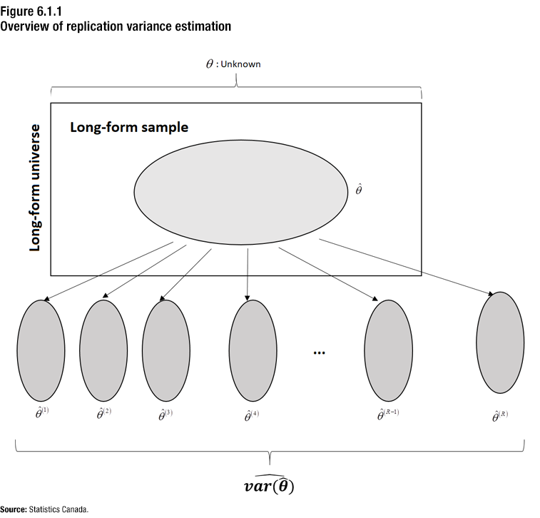
Figure 6.1.1 gives an overview of replication variance estimation when $R$ samples are used.

The following are defined:

• theta, $\theta$, the true value of the characteristic in the population, which can be a total, an average, a quantile, etc.
• theta hat, $\widehat{\theta }$, the value of $\theta$ estimated using the main weights
• theta hat $r$, ${\widehat{\theta }}^{(r)}$, the value of $\theta$ estimated using the replication weights $r$, $r=1,\mathrm{...},R$
• theta hat bar, $\overline{\widehat{\theta }}$, the average value of the $R$ replication estimates ${\widehat{\theta }}^{(r)}$
• $\widehat{\mathrm{var}}(\widehat{\theta })$, the estimated value of the variance of $\widehat{\theta }$.

6.2 Variance estimator

The replicate estimator chosen for the long-form sample survey was derived from Fay’s balanced half-sample method (Judkins 1990). This method determines the creation of replicates, the calculation of replicate weights and the multiplication factor used to estimate variance.

To produce variance estimates for the long-form sample estimates, two sets of replicate weights were created: the first had 32 replicate weights and the second had 100 replicate weights. The set of 32 replicate weights was produced to estimate the standard errors of standard products that are calculated under operational constraints (i.e., the need to publish a large number of confidence intervals within a reasonable time frame). The set of 100 replicate weights was made available to Statistics Canada analysts and research data centre analysts who have access to microdata to provide more precise variance estimators.

The replication variance estimator can be calculated in two ways, one of which is more conservative than the other. The first method consists of taking the sum of the squared differences between the replication estimates, ${\widehat{\theta }}^{(r)}$, and the average of the replication estimates, $\overline{\widehat{\theta }}$. The second method consists of taking the sum of squared differences between the replication estimates, ${\widehat{\theta }}^{(r)}$, and the estimate from the original sample, $\widehat{\theta }$. With both methods, the sum of squared differences is multiplied by a certain factor. The second method, which uses the estimate from the primary sample, is more conservative. In the computer system used to publish statistics, the variance estimator is calculated using the estimate from the primary sample.

For example, two variance estimators of an estimator $\widehat{T}$ of a total $T$ from a set of $R$ replicates are given in the equations below:

where

The final weight of the sample is represented by $w_k$, $w_k{}^{(r)}$ is the final weight of replicate $r$, $y_k$ is the value of characteristic $y$ for unit $k$, and $s$ is the long-form sample.

The number of degrees of freedom of the variance estimator is approximated by the number of squared differences ${\left({\widehat{T}}^{(r)}-\overline{\widehat{T}}\right)}^2$ for the variance estimator, i.e., 32 or 100. The number of degrees of freedom gives an idea of the precision of the variance estimator and is used in calculating confidence intervals for long-form estimates. See Chapter 7 for more details.

6.3 Replicate weight adjustment

6.3.1 Mail-out and list/leave collection units

As mentioned in Section 6.2, replicate weights were calculated for all long-form sample households. The replicates were partially balanced. They were balanced by resampling strata, which were created by combining CUs to obtain 600 to 1,800 households per resampling stratum.

Fay’s modified balanced half-sample method, as described by Rao and Shao (1999), requires an epsilon value in the calculation of replicate weights to control the perturbation of the replicate weights. This perturbation results in all sampled households participating in every replicate, unlike other more popular replication methods. This facilitates the calibration of the replicate weights and, occasionally, the calculation of point estimates for each replicate (e.g., the denominator of a ratio estimator for a given replicate will not have a nil value if the corresponding denominator was not nil with the final weight). Adding an epsilon factor to the calculation of replicate weights meant the large survey fraction used to select the long-form sample could be taken into account. The technical details of the variance estimation process were provided by Devin and Verret (2016).

The replicate weights underwent the same adjustments as the primary sample design weight. They were adjusted for coverage and total non‑response following the same methodology that was used for the primary sample weight (see Section 4.4). The resulting replicate weights were then calibrated to census counts, once again following the same methodology that was used for the main weight (see Section 4.5).

6.3.2 Collection units in First Nations communities, Métis settlements, Inuit regions and other remote areas^{Note 2}

As described in Chapter 2, all the households in First Nations communities, Métis settlements, Inuit regions and other remote areas CUs were selected with certainty. As such, they originally had a design weight equal to 1. A coverage adjustment was not needed. All these households were selected for the long-form questionnaire, and therefore differential coverage between the short-form and long-form questionnaire could not occur. Total non‑response in these areas was treated with the process of whole household imputation (WHI), described in Chapter 3. In other words, the data of a non‑responding household were replaced by the data of another responding household from the same CU (except for geography variables, which were known for non‑respondents). As a consequence, reweighting for households in those CUs was not needed.

Calibration was not needed in these areas, because the long-form questionnaire was a census. Consequently, all households in First Nations communities, Métis settlements, Inuit regions and other remote areas CUs maintained their original weight equal to 1 in the final weighting scheme.

Although sampling variability did not occur for households in - First Nations communities, Métis settlements, Inuit regions and other remote areas CUs, WHI variability did occur. Variance estimation in these areas was computed using a similar method to that of the rest of the country, with the following exceptions. First, the response probability by household size combination in each census division was estimated as the number of responding households divided by the number of in-scope households. Then, the base replicate weights were created as in the rest of the country, except that all respondents for which the response probability was equal to 1 were placed in every replicate. Respondents with estimated response probabilities less than 1 were not considered certainties and were treated as sampled elements (i.e., they were randomly divided among the replicates). Non‑respondent households imputed by WHI were also divided among replicates, and each one was assigned the replicate inclusion indicator corresponding to its donor in a manner similar to that of Shao and Tang (2011). This caused the weights to vary from one replicate to the other. Finally, the replicate weights were calibrated to the number of households and number of persons in the SADA. As a result, the estimated variance of those two quantities was equal to 0 at the SADA level and at more aggregate levels, such as Canada (since those two constraints are mandatory in the rest of the country).

• Previous
• Next