Sampling and Weighting Technical Report, Census of Population, 2016
6. Variance estimation

The error in an estimate is the difference between the estimate and the actual value of what is being estimated. There are several sources of error in the long-form sample survey, including sampling error and total non-response error. Sampling error stems from the fact that the estimates are based on observations from a sample and not from the Census of Population. Total non-response error occurs when households selected in the sample do not respond to the survey.

Error has a random component, measured by variance, and a systematic component, measured by bias. Variance measures how much the estimate varies from the average that would result from hypothetical repetitions of the survey process. Variance can be estimated using data from the sample. Bias is the difference between the average estimate that would result from hypothetical repetitions of the survey process and the actual value of the characteristic being estimated. The sampling and estimation methods used in the long-form sample survey produce a negligible bias.

Some estimation methods are more precise than others in estimating a particular characteristic of the population, so they can affect error. The estimated variance can be used to produce several quality indicators that are often used to measure the accuracy of an estimate. For example, it can be used to calculate standard errors, confidence intervals and coefficients of variation. Standard error was the quality indicator produced for the 2016 Census long-form estimates. Standard error corresponds to the square root of the variance.

These measures of variability must be carefully distinguished from other measures of quality that are not, strictly speaking, measures of variability. Examples of such measures are the final response rates presented in section 3.11 and the global non-response rate to the 2016 Census long-form questionnaire. The response rate is an indicator of the risk associated with household non-response error. The global non-response rate is an indicator of the risk of error attributable to household non-response and item non-response. For more information, see Chapter 11 of the Guide to the Census of Population, 2016 (Statistics Canada 2017).

Since the long-form sample is geographically stratified into take-some strata (mail-out and list/leave CUs) and take-all strata (canvasser CUs), two variance estimators are used. The first variance estimator is used to estimate the variance in take-some geographic areas (see section 6.3.1), and the second estimator is used to estimate the variance attributable to total non-response in take-all areas (see section 6.3.2). For the remainder of this chapter, the term variance is used to designate the sampling and total non-response variance in take-some geographic areas or the total non-response variance in take-all areas.

Standard errors for various estimates and geographic areas can be viewed or downloaded from the Census Profile Standard Error Supplement, Canada, provinces, territories, census divisions (CDs) and aggregate dissemination areas (ADAs), 2016 Census. The sampling and estimation methods used for the 2016 long-form survey are different from those used for the 2011 National Household Survey (NHS). Since the size and impact of non-response were very different in 2011, they affected estimate variability. For more information, refer to the methodological note comparing standard errors for 2016 estimates with those for 2011 and 2006 estimates for some variables.

6.1 Elements to consider in choosing a variance estimation method

A very high number of diverse estimates were produced, and quality indicators for these estimates needed to be established within a reasonable timeframe. As a result, a resampling variance estimator was used, derived from the modified partially balanced repeated replication method (Judkins 1990). The method consists of drawing samples (or replicates) from the original sample. Weights are calculated for each replicate, and the weights undergo the same coverage, non-response and calibration adjustments as the original sample. The resulting weights are called replicate weights. Estimates are then produced for each replicate, and the variance is estimated using replicate estimates and the average of these estimates.

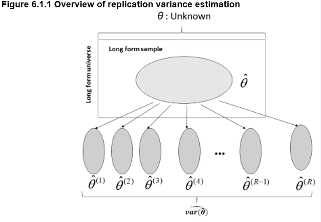
Figure 6.1.1 gives an overview of replication variance estimation when R samples are used.

Figure 6.1.1 gives an overview of the replication variance estimation methodology used in the 2016 Census. The replication variance estimation method simulates the selection of several samples to estimate sampling variance.

More specifically, the figure shows the long-form questionnaire universe representing the population of interest and the long-form questionnaire sample. The sample is situated within the universe to indicate whether it corresponds to a subset of the population of interest. This sample is used to estimate a characteristic of the population of interest, such as the number of people who are members of a visible minority. The theta symbol is used to represent the true value of this characteristic. A circumflex on the theta indicates that the value is an estimate of this characteristic. This value is known as theta hat.

The R other samples placed outside the universe are linked to the long-form questionnaire sample with arrows. The arrows indicate that these samples are taken from the long-form questionnaire sample. The characteristic of interest is re-estimated based on these R sub-samples. The theta hat R values, referred to as theta hat one, theta hat two, up to theta hat R, are used to calculate the estimated theta hat variance.

In this figure, we define:

• theta, $\theta$, the true value of the characteristic in the population, which can be a total, an average, a quantile, etc.;
• theta hat, $\widehat{\theta }$, the value of $\theta$ estimated using the main weights;
• theta hat r, ${\widehat{\theta }}^{(r)}$, the value of $\theta$ estimated using the replication weights r, r=1, ..., R;
• theta hat bar, $\overline{\widehat{\theta }}$, the average value of the R replication estimates ${\widehat{\theta }}^{(r)}$ and
• $\mathrm{v}\widehat{a}r(\widehat{\theta })$, the estimated value of the variance of $\widehat{\theta }$.

6.2 Variance estimator

The replicate estimator chosen for the long-form sample survey was derived from Fay's balanced half-sample method (Judkins 1990). This method determines the creation of replicates, the calculation of replicate weights and the multiplication factor used to estimate variance.

To produce variance estimates for the long-form sample estimates, two sets of replicate weights were created: the first had 32 replicate weights and the second had 100 replicate weights. The set of 32 replicate weights was produced to estimate the standard errors of standard products that are calculated under operational constraints (i.e., the need to publish a large number of standard errors within a reasonable timeframe). The set of 100 replicate weights was made available to Statistics Canada analysts, research data centre analysts who have access to microdata and users who request custom products, to provide more precise variance estimators.

The replication variance estimator can be calculated in two ways, one of which is more conservative than the other. The first method consists of adding the squared differences between the replication estimates, ${\widehat{\theta }}^{(r)}$, and either the average of the replication estimates, $\overline{\widehat{\theta }}$, or the estimate from the primary sample, $\widehat{\theta }$, and multiplying this sum by a certain factor. The second method, which uses the estimate from the primary sample, is more conservative. In the Computer-assisted Product Specification System used to publish statistics, the variance estimator is calculated using the average of the replication estimates.

For example, two variance estimators to estimate a total from a set R of replicates are given in the equations below:

$$\begin{array}{l}V\widehat{a}{r}_1\left(\widehat{T}\right)=\frac{1}{\raisebox{1ex}{$R$}\!\left/ \!\raisebox{-1ex}{$2$}\right.}{\displaystyle \sum _{r=1}^{\text{R}}{\left({\widehat{T}}^{(r)}-\overline{\widehat{T}}\right)}^2},\\ V\widehat{a}{r}_2\left(\widehat{T}\right)=\frac{1}{\raisebox{1ex}{$R$}\!\left/ \!\raisebox{-1ex}{$2$}\right.}{\displaystyle \sum _{r=1}^{\text{R}}{\left({\widehat{T}}^{(r)}-\stackrel{}{\widehat{T}}\right)}^2}\end{array}$$

where

$$\begin{array}{l}\widehat{T}={\displaystyle {\sum }_{k\in s}{w}_k}{y}_k,\\ {\widehat{T}}^{(r)}={\displaystyle {\sum }_{k\in s}{w}_k^{(r)}}{y}_k,\text{and}\\ \overline{\widehat{T}}={\displaystyle {\sum }_{r=1}^R{\widehat{T}}^{(r)}}/\text{R}.\end{array}$$

The final weight of the sample is represented by $w_k$ , $w_k^{(r)}$ is the final weight of replicate r , $y_k$ is the value of characteristic y for unit k, and s is the long-form sample.

The number of degrees of freedom of the variance estimator is approximated by the number of squared differences ${\left({\widehat{T}}^{(r)}-\overline{\widehat{T}}\right)}^2$ for the variance estimator, i.e., 32 or 100. The number of degrees of freedom gives an idea of the precision of the variance estimator and is used in calculating confidence intervals for long-form estimates. Since the method used to estimate the variance of the estimate can use few replicates, Student's law of probability was used to determine the quantile of the confidence level to be used in calculating the interval. In cases where the number of households participating in the estimate is larger than R, the number of degrees of freedom should be R. In cases where the number of households is less than R but equal to or greater than 20, the number of degrees of freedom corresponds to the number of households. Producing confidence intervals when there are fewer than 20 households is not recommended.

6.3 Replicate weight adjustment

6.3.1 Mail-out and list/leave collection units

As mentioned in section 6.2, replicate weights were calculated for all long-form sample households. The replicates were partially balanced. They were balanced by resampling strata, which were created by combining CUs to obtain 600 to 1,800 households per resampling stratum.

Fay's modified balanced half-sample method, as described by Rao and Shao (1999), requires an epsilon value in the calculation of replicate weights to control the perturbation of the replicate weights. This perturbation results in all sampled households participating in every replicate, unlike other more popular replication methods. This facilitates the calibration of the replicate weights and, occasionally, the calculation of point estimates for each replicate (e.g., the denominator of a ratio estimator for a given replicate will not have a nil value if the corresponding denominator was not nil with the final weight). Adding an epsilon factor to the calculation of replicate weights meant the large survey fraction used to select the long-form sample could be taken into account. The technical details of the variance estimation process were provided by Devin and Verret (2016).

The replicate weights underwent the same adjustments as the primary sample design weight. They were adjusted for coverage and total non-response following the same methodology that was used for the primary sample weight (see section 4.4). The resulting replicate weights were then calibrated to census counts, once again following the same methodology that was used for the primary weight (see section 4.5).

6.3.2 Indian reserve^{Note 1} and canvasser enumeration collection units

As described in Chapter 2, all the households in Indian reserve and canvasser enumeration CUs were selected with certainty. As such, they originally had a design weight equal to 1. A coverage adjustment was not needed. All these households were selected for the long form, and therefore differential coverage between the short and long form could not occur. Total non-response in these areas was treated with the process of whole household imputation (WHI), described in Chapter 3. In other words, the data of a non-responding household were replaced by the data of another responding household from the same CU (except for geography variables, which were known for non-respondents). As a consequence, reweighting for households in Indian reserve and canvasser enumeration CUs was not needed.

Calibration was not needed in these areas, because the long form was a census. Consequently, all households in Indian reserve and canvasser enumeration CUs maintained their original weight equal to 1 in the final weighting scheme. For more information on incompletely enumerated Indian reserves and Indian settlements, please refer to Appendix 1.2 of the Guide to the Census of Population, 2016, Catalogue no. 98-304-X.

Although sampling variability did not occur for households in Indian reserve and canvasser enumeration CUs, WHI variability did occur. Variance estimation in these areas was computed using a similar method to that of the rest of the country, with the following exceptions. First, the response probability by household size combination in each census division was estimated as the number of responding households divided by the number of in-scope households. Then the base replicate weights were created as in the rest of the country, except that all respondents for which the response probability was equal to 1 were placed in every replicate. Respondents with estimated response probabilities less than 1 were not considered certainties and were treated as sampled elements (i.e., they were randomly divided among the replicates). Non-respondent households imputed by WHI were also divided among replicates, and each one was assigned the replicate inclusion indicator corresponding to its donor in a manner similar to that of Shao and Tang (2011). This caused the weights to vary from one replicate to the other instead of the values. Finally, the replicate weights were calibrated to the number of households and number of persons in the SADA. As a result, the estimated variance of those two quantities was equal to 0 at the SADA level and at more aggregate levels, such as Canada (since those two constraints are mandatory in the rest of the country).

Note

• Previous
• Next